Let image complexity decide the groups.
Control how much detail the mixture keeps.
Full-covariance Gaussian mixtures with stronger model-selection penalties, Bayesian concentration priors, and orthogonal varimax rotation. Compare counts, their repeatability, and the same image boundaries.
10 images per domainWhole · local 5%, 10%, 20%3 or 16 retained dimensionsFour flips + 75% overlap for local featuresFull covariance throughoutPractical choice after inspecting the maps
Keep automatic K-means as the default reference. For full-covariance GMM on 16 retained dimensions, λ=4 is a moderate count regularization choice and λ=8 is a coarser alternative. For the three-dimension representation, λ=8 places more images in the preferred 4–6 range. These are operational choices from this collection, rather than a universal optimum.
A concrete counterexample is fungal_network_01: the inspected local 10%, 16-axis K-means map retains fine radial branching texture, while GMM at λ=4 and λ=8 merges much of it into broad regions. In PMID microscopy, lower penalties can split a single organism into several feature groups. Count reduction and repeatability must therefore be considered alongside the biological structures of interest. No reviewed object masks were used.
What changes when the penalty becomes stronger?
Each row uses the same fitted candidate mixtures and the same fitting locations. Only λ changes. λ=1 is ordinary BIC; higher values deliberately place more weight on model simplicity.
Distribution of selected K
Each image and the mean
Selected K is the mixture component count. Image maps also report occupied groups and the largest group’s area; fewer groups do not imply more balanced areas.
Does a sparse Bayesian prior reduce the groups?
A separate BayesianGaussianMixture experiment, with a maximum of 12 components and a Dirichlet-process concentration prior α. All other priors and fitting locations are held fixed. This is a different estimator from strengthened BIC.
Distribution across concentration settings
Each image and the mean
Weights are mixture proportions in feature space. They are not species probabilities. An occupied group is any component receiving at least one maximum-responsibility assignment on the full feature grid.
Does the choice repeat across spatial samples?
Local 10% features, earlier frozen ten-image subset with two images per domain. Three resamples use different two-thirds selections of 8×8 spatial blocks, with 8,192 fitting locations each. Every resample independently fits K=1…12 and selects K for every λ.
Adjusted Rand index (ARI) compares the selected partitions on common probe locations. 1 means identical partitions; it measures agreement, not segmentation accuracy. High λ can achieve high agreement simply by collapsing everything into one group. Shared DINO context and crop overlap remain across block boundaries. This section always summarizes its fixed ten-image subset; the dataset filter above does not change it.
Inspect the same image across settings
Original PCA colors and varimax colors display three axes. Clustering uses all selected retained axes. The original PCA color calibration is retained as a reference; varimax colors use a shared 2nd–98th percentile stretch across the four retained feature approaches for that image. Independent channel stretching means visible color contrast is not identical to the distance metric used for clustering.
Click any map to center all panels on that location. Colors align to the K-means reference where possible; numerical labels and colors have no biological identity. Preview resolution resolves the retained 256-cell grid, and the label arrays are downloadable.
Selection score for this image
Counts across all settings for this image
How the experiment was calculated
The stronger penalty
Sλ(K) = −2 log LK + λ pK log n
For d retained dimensions and full covariance, pK = K[d + d(d+1)/2] + K − 1. Each image/feature/dimension case fits all K=1…12 on the identical fixed sample of 8,192 or fewer feature locations. Candidates must converge. Select the lowest score, with smaller K breaking an exact tie. Ordinary BIC corresponds to λ=1; λ=2,4,8,16,32,64 are explicit additional regularization preferences.
All candidate fits use full covariance, three initializations, seed 42, covariance diagonal regularization 10−5, convergence tolerance 0.001, 300 iterations and a 600-iteration continuation if needed. Candidates were refitted in float64 for internally consistent scoring. The feature grid and PCA subspace were reused.
Bayesian concentration and component counts
BayesianGaussianMixture uses variational inference with full covariance and a maximum of 12 components. Concentration α=0.001,0.01,0.1,1,10,100 is varied; mean precision prior is 1, covariance prior is the empirical full covariance, and the covariance degrees-of-freedom prior equals d. One initialization, seed 42, tolerance 0.001, 500 iterations with a 1,000-iteration continuation; difficult cases receive a further 5,000-iteration continuation at the same tolerance. This experiment isolates concentration sensitivity; it is not an exhaustive optimization of Bayesian priors.
Occupied group count, components with weight ≥1%, and groups with area ≥1% describe different properties. None of the thresholds deletes or reassigns groups. All map locations receive a maximum-responsibility assignment.
Varimax, projection scores, and rotational invariance
The original per-image PCA basis B has 768 rows and d retained columns. Varimax optimizes the PCA projection-weight loadings with Kaiser row normalization, five deterministic starts, and SVD updates. The row normalization is used only for optimizing the rotation. The original basis and unwhitened scores are then rotated as Brot = B R and Xrot = X R, with RᵀR=I. This uses projection-weight loadings; the alternative covariance-loading / standardized factor-score convention is not used.
All d axes are retained after rotation. Euclidean distances and the represented subspace remain unchanged. Rotated scores can be correlated and their axes are not ordered by explained variance. A full covariance transforms as RᵀΣR, so pointwise likelihoods, responsibilities, and selected K remain the same under an exact reparameterization. Varimax can change which patterns appear in RGB but cannot itself improve Euclidean K-means or full-covariance GMM partitions.
Sampling and what these results establish
The collection contains ten previously selected examples per domain. Local 5/10/20% crops use 384×384 enlargement, inverse-aligned four-flip averaging, approximately 75% overlap, and Hann blending. Whole-image features use the existing working image/window. The feature grid has an aspect-preserving longest side of 256 locations. Features are unwhitened; spatial coordinates and RGB are not clustering inputs.
K-means remains an automatic reference using the earlier spatial-fold silhouette rule, selecting the candidate closest to five within one standard error of the best score. It therefore already has a preference toward five. Its labels are preserved under orthogonal rotation, verified by independent refits.
Interpolated locations and overlapping context are correlated. Classical BIC’s independent-observation assumptions do not hold exactly here. Penalty sensitivity and blocked repeatability support a practical clustering choice, but establish neither species counts nor leaf/organism segmentation accuracy. A universal λ or α is not inferred.
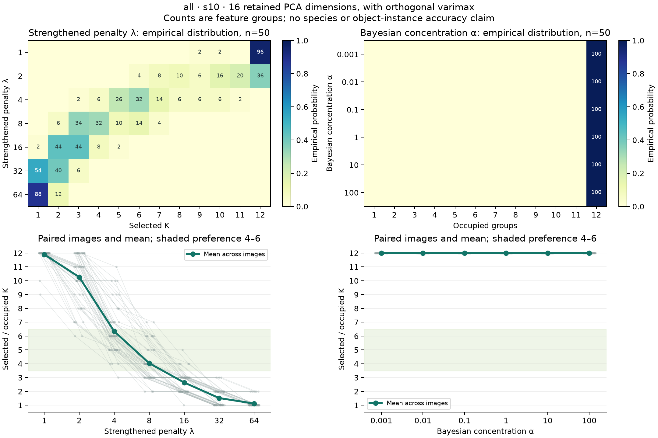
Scientific figure downloads summarize the full 50-image collection for the selected feature/dimension setting. The interactive charts honor the dataset filter.