A full-cohort analysis of detected plant families, spatial image patterns and common-coordinate DINO features across Feßbach, Heidesheim, Rettmer and Ribbeck.
Taxonomic results describe supported model detections. Species and genus identifications have already been promoted to their recorded family and combined with direct family identifications. A family is resolved in 342 photos; 97 are unresolved. The median family-assigned area is 20.8% of eligible image area after this promotion (direct family identifications alone would give 9.35%). Of 342 resolved photos, 281 contain just one detected family. These results provide a conservative detected-family baseline; they do not establish the full biological diversity in each photograph.
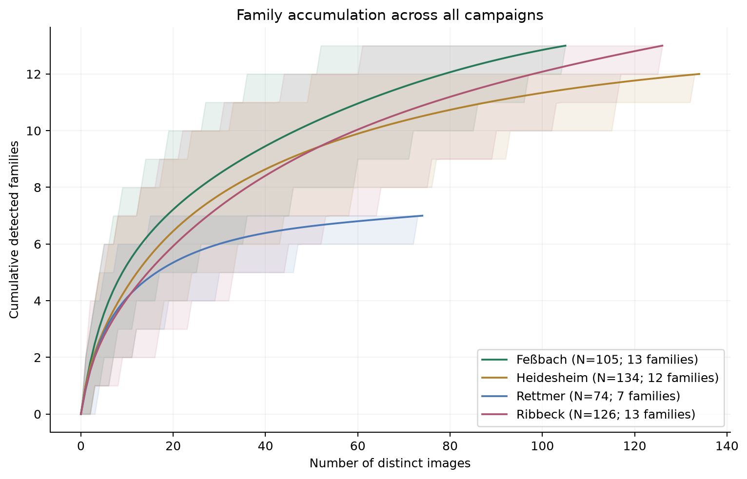
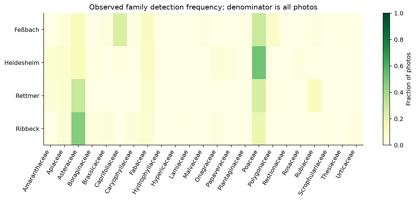
Feßbach has the most even detected family composition and the highest mean within-image DINO diversity. Heidesheim is dominated by Poaceae detections; Ribbeck by Asteraceae. Rettmer has seven detected families and the largest unresolved fraction. Equal-effort comparison at 74 images retains the order Feßbach, Ribbeck, Heidesheim, Rettmer.
Site
Distinct photos
Family-resolved
Detected families γ0
Expected families at 74 photos
Structural α
Structural β
Structural γ
Feßbach
105
87 / 105
13
11.77
0.389
0.110
0.499
Heidesheim
134
111 / 134
12
10.51
0.360
0.122
0.482
Rettmer
74
50 / 74
7
7.00
0.370
0.112
0.481
Ribbeck
126
94 / 126
13
10.88
0.376
0.121
0.497
Structural values are continuous feature-variance proxies in DINO space, with equal weight per photo. They are not counts of plant species or measured canopy layers.
Workflow distinction. The whole-cohort calculations use the existing full-frame DINO patch cache and the existing taxonomic region evidence at support 0.7. The adopted 5%/10% local-crop workflow, with 75% overlap, automatic K-means and full-covariance GMM (λ = 4), was benchmarked on 10 MOIN photos within a 50-image multi-dataset experiment. The new photo-view batch is generating 5% maps for the full cohort; availability is shown in the ranking browser. The biodiversity summaries remain based on the cached full-frame features and existing family evidence. Existing taxonomic regions were produced with the older AnyUp workflow; the report preserves that provenance.
1. Per-image diversity and rankings
The primary structural ranking uses exact within-photo Rao Q from all eligible native DINO patches. The primary taxonomic ranking uses effective detected families, q1 = exp(Shannon entropy), weighted by accepted family-region areas and conditioned on family-resolved area. A mixed-rank named-label score and the earlier structural composite remain available as sensitivity views.
Ranks are assigned across the full cohort. Equal family diversity receives a tied rank; unresolved images have no family-diversity rank. High scores can be driven by visible ground, senescence, viewpoint or unresolved regions, so the photo viewer shows assignment coverage alongside each score.
Highest within-image DINO diversity
Highest effective detected-family diversity
Click any ranked photo to compare DINO maps. The photo viewer presents plain PCA, PCA-varimax, automatic K-means and λ=4 GMM in matched whole-frame and 5% crop columns.
Loading map availability…
Photo
Site / campaign
Structural rank
Rao Q
Family rank
Detected families
q1
Family-assigned area
DINO maps
Click a photo to inspect its image, family hypotheses, configuration map, coordinates, original source path, metadata and duplicate aliases.
2. Cumulative family coverage
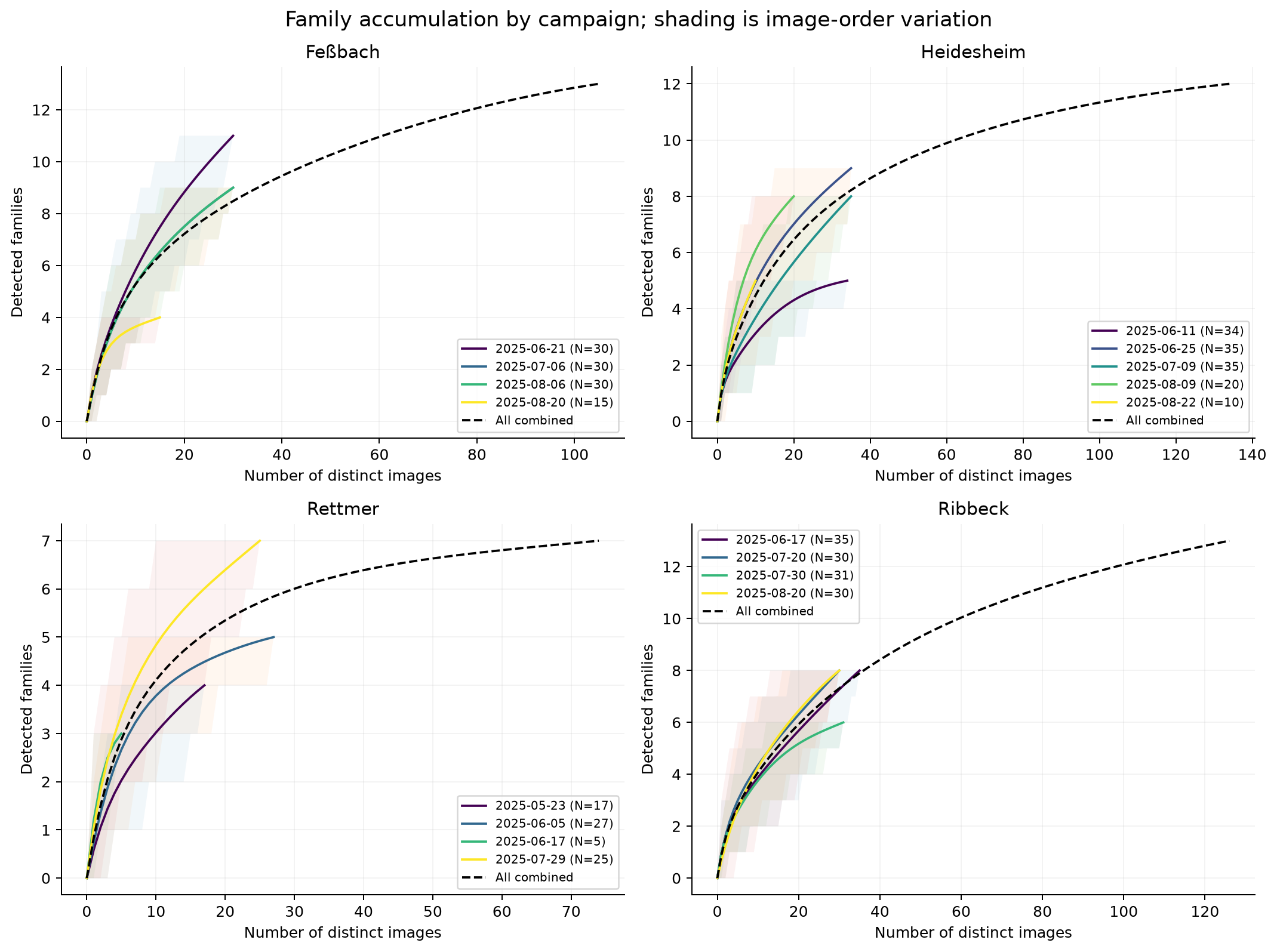
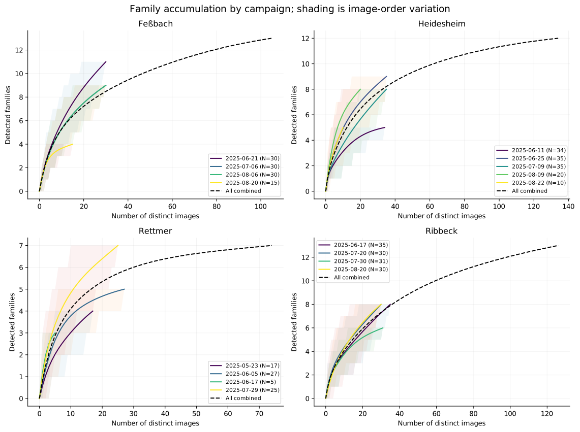
Curves count distinct detected families as image effort increases. The line is the exact expected richness over all possible subsets of each size. Shading spans the central 95% of 1,000 randomized image orders, describing order sensitivity within this observed collection. Every distinct photo counts as effort, including family-unresolved photos.
Exact expected cumulative detected-family richness at each image effort; shaded bands describe randomized order variation. Download SVG
The dashed curve combines all campaigns at a site. Campaigns have unequal sample sizes; compare curves at common image effort.
Only Rettmer includes spring (May); all other images are summer (June–August). Consequently, a four-site spring-versus-summer comparison cannot be estimated from this collection. Individual campaigns and month groupings preserve the finer sampling structure.
Campaign inventory and estimator limits
Site
Sampling campaign
Photos
Detected families
Feßbach
2025-06-21
30
11
Feßbach
2025-07-06
30
9
Feßbach
2025-08-06
30
9
Feßbach
2025-08-20
15
4
Heidesheim
2025-06-11
34
5
Heidesheim
2025-06-25
35
9
Heidesheim
2025-07-09
35
8
Heidesheim
2025-08-09
20
8
Heidesheim
2025-08-22
10
5
Rettmer
2025-05-23
17
4
Rettmer
2025-06-05
27
5
Rettmer
2025-06-17
5
3
Rettmer
2025-07-29
25
7
Ribbeck
2025-06-17
35
8
Ribbeck
2025-07-20
30
8
Ribbeck
2025-07-30
31
6
Ribbeck
2025-08-20
30
8
Folder dates define campaigns. Seventeen Rettmer photos in the 5 June folder have EXIF dates of 3 or 4 June; their conflict is retained. Chao2 lower bounds and incidence sample-coverage estimates are supplied in the data, but an estimated coverage of 1.0 is not evidence of complete vegetation identification. Rettmer has a singleton/doubleton boundary case, and missing model identifications are outside the estimator’s assumptions. The report therefore emphasizes observed-family accumulation rather than a biological completeness claim. Rarefaction and completeness estimation follow the framework discussed by Chao et al. (2014).
3. Site diversity, composition and configuration
Site
α0: mean detected families¹
α1: effective families¹
γ1: pooled effective families¹
β1 = γ1/α1¹
Within-campaign Sørensen²
Turnover²
Nestedness²
Feßbach
1.195
1.119
6.445
5.759
0.774
0.747
0.027
Heidesheim
1.171
1.096
4.299
3.923
0.573
0.534
0.039
Rettmer
1.240
1.141
4.656
4.080
0.705
0.641
0.064
Ribbeck
1.191
1.116
4.186
3.751
0.591
0.540
0.051
¹ Family-resolved photos only, conditional family-area proportions, equal photo weights. γ1 is exp(entropy of pooled proportions); α1 is exp(mean within-photo entropy); β1 = γ1/α1. α0 is mean detected richness. ² Pairwise means between family-resolved photos from the same campaign; these describe spatial image heterogeneity at sampling time, including different views of a plot. Repeated plots and unknown physical footprints limit independence. See Jost (2007) for multiplicative diversity partitioning.
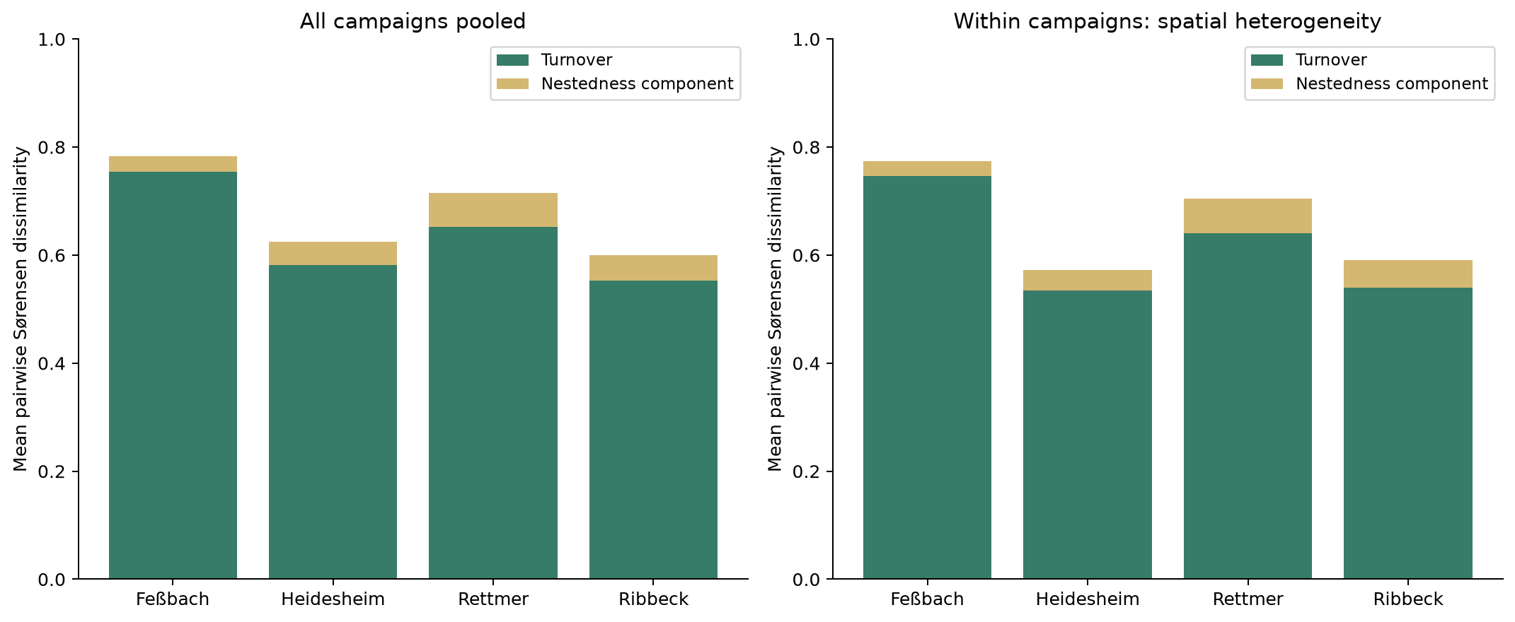
Family detection frequency, with all photos in the denominator. Unresolved photos count as no detection, not biological absence. Download SVGDetected compositional dissimilarity partitioned into turnover and nestedness: pooled campaigns and within-campaign spatial comparisons. Download SVG
Feßbach
13 detected families; γ1 = 6.44 effective families. Poaceae appears in 31/87 family-resolved photos and Caprifoliaceae in 26/87. Asteraceae and Fabaceae also contribute. Within-campaign Sørensen dissimilarity is 0.774, the highest of the four sites, driven mainly by family replacement. Structural α is also highest (0.389).
Heidesheim
12 detected families; γ1 = 4.30. Poaceae appears in 69/111 resolved photos (62%), with Asteraceae and Fabaceae next. Within-campaign dissimilarity is 0.573, the lowest of the four sites. Its lower mean structural α (0.360) coexists with the largest structural β (0.122), indicating relatively less within-photo variation but more variation between photo means.
Rettmer
7 detected families; γ1 = 4.66. Asteraceae and Poaceae appear in 22/50 and 19/50 resolved photos; Rubiaceae appears in 8/50. Within-campaign dissimilarity is 0.705. With 24/74 photos unresolved (32%), the low observed richness cannot establish that the site is biologically poorer. Its spring sampling is unique in this dataset.
Ribbeck
13 detected families; γ1 = 4.19. Asteraceae appears in 59/94 resolved photos (63%), followed by Poaceae (22/94). Within-campaign dissimilarity is 0.591. The resolved masks have more components than Feßbach or Heidesheim, but their lower resolved coverage and different photo footprints prevent an ecological fragmentation claim.
Turnover accounts for most detected compositional dissimilarity at every site; nestedness is smaller. Pooling campaigns also mixes temporal changes with spatial differences, which is why the same-campaign comparison is shown separately. The Sørensen turnover/nestedness decomposition follows Baselga (2010).
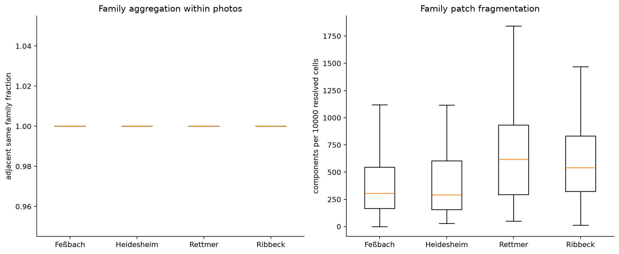
Configuration within the photographed footprint
Site
Same-family neighbor joins
Components / 10,000 resolved cells
Resolved image-grid fraction
Mean configuration distance³
Feßbach
99.1%
421
27.5%
0.163
Heidesheim
99.2%
450
30.1%
0.176
Rettmer
99.1%
686
19.4%
0.182
Ribbeck
99.1%
620
18.8%
0.161
Exploratory configuration of unambiguous family regions; incomplete coverage and coarse masks affect both descriptors. Download SVG
³ Gower distance averages absolute differences in range-scaled same-family neighbor joins, component density and resolved grid fraction. Masks include only unambiguous, accepted single-family regions; ambiguous regions are unresolved. They are sampled on an aspect-preserving grid with longest side 256. Same-family joins are about 99% at all sites, partly reflecting the coarse, smooth region masks. Components and their densities depend on support coverage and grid resolution. These are exploratory image configuration descriptors, not mapped field patches.
Metadata join to 313 photos at Feßbach, Heidesheim and Rettmer. Ribbeck plot keys are inferred from filenames and marked accordingly. There are 359 between-campaign image comparisons sharing a recorded plot key; multiple orientations can generate several comparisons per plot. Those comparisons are exported for descriptive follow-up. Geographic coordinates and calibrated plot footprints were not recovered, so distance-decay and true geographic beta diversity are not estimated here.
4. Community NMDS and photo exploration
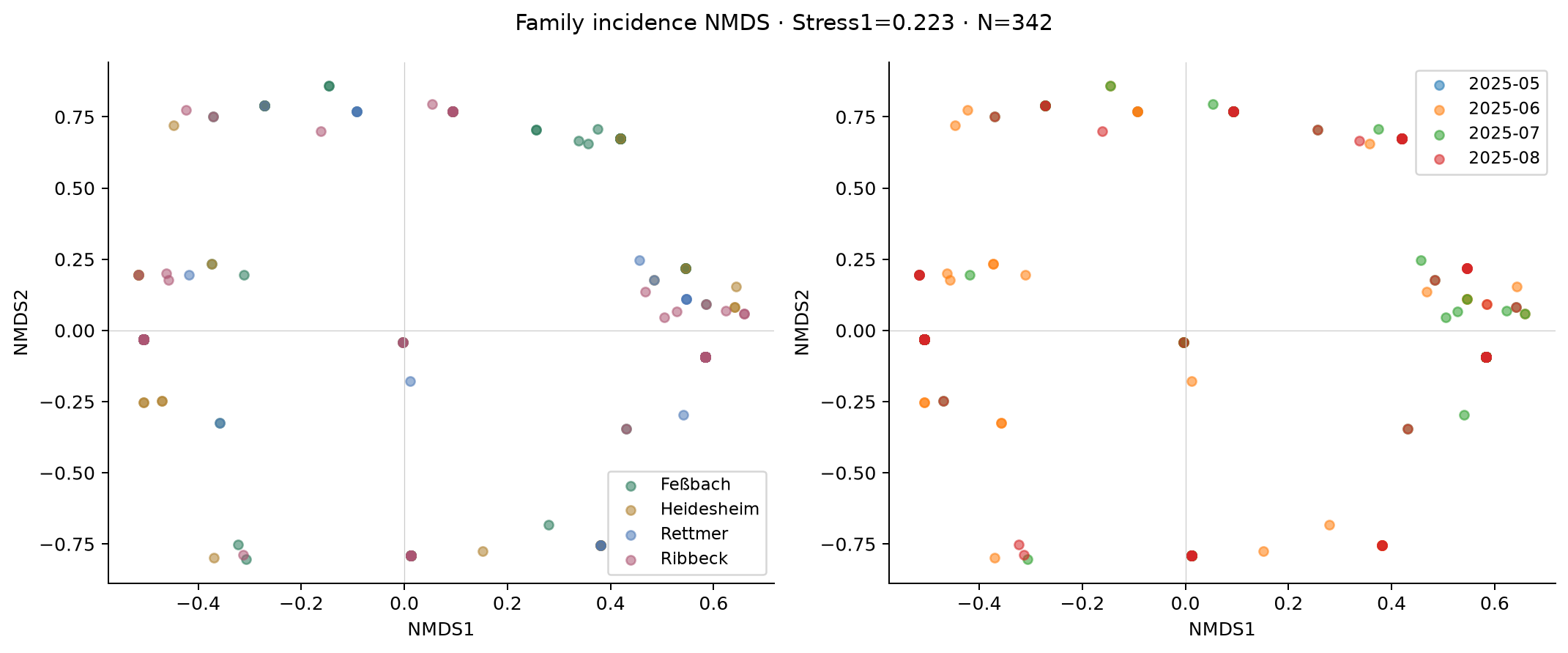
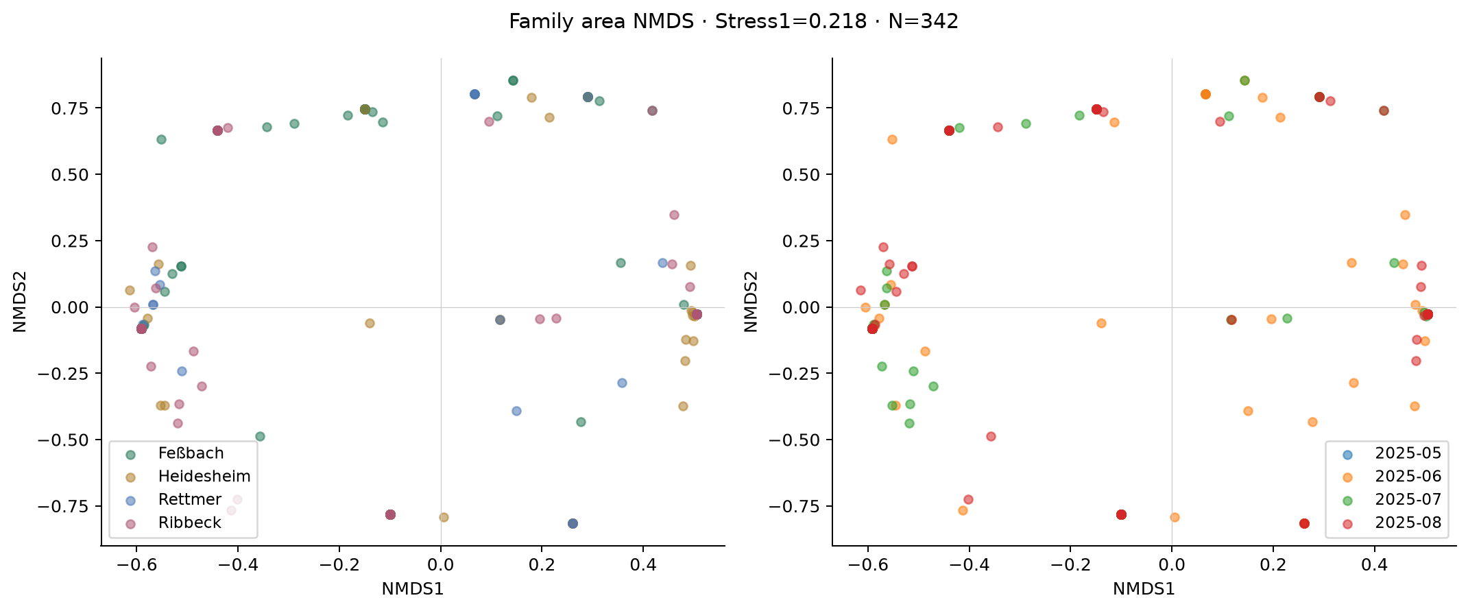
Family incidence uses Jaccard dissimilarity; conditional family-area composition uses Bray–Curtis. Both ordinations include 342 family-resolved photos. Identical profiles share coordinates: there are only 49 distinct incidence profiles and 75 distinct area profiles. Many points coincide because a photo often has one detected family. Thus an apparently separated group may reflect that family rather than a distinct whole community.
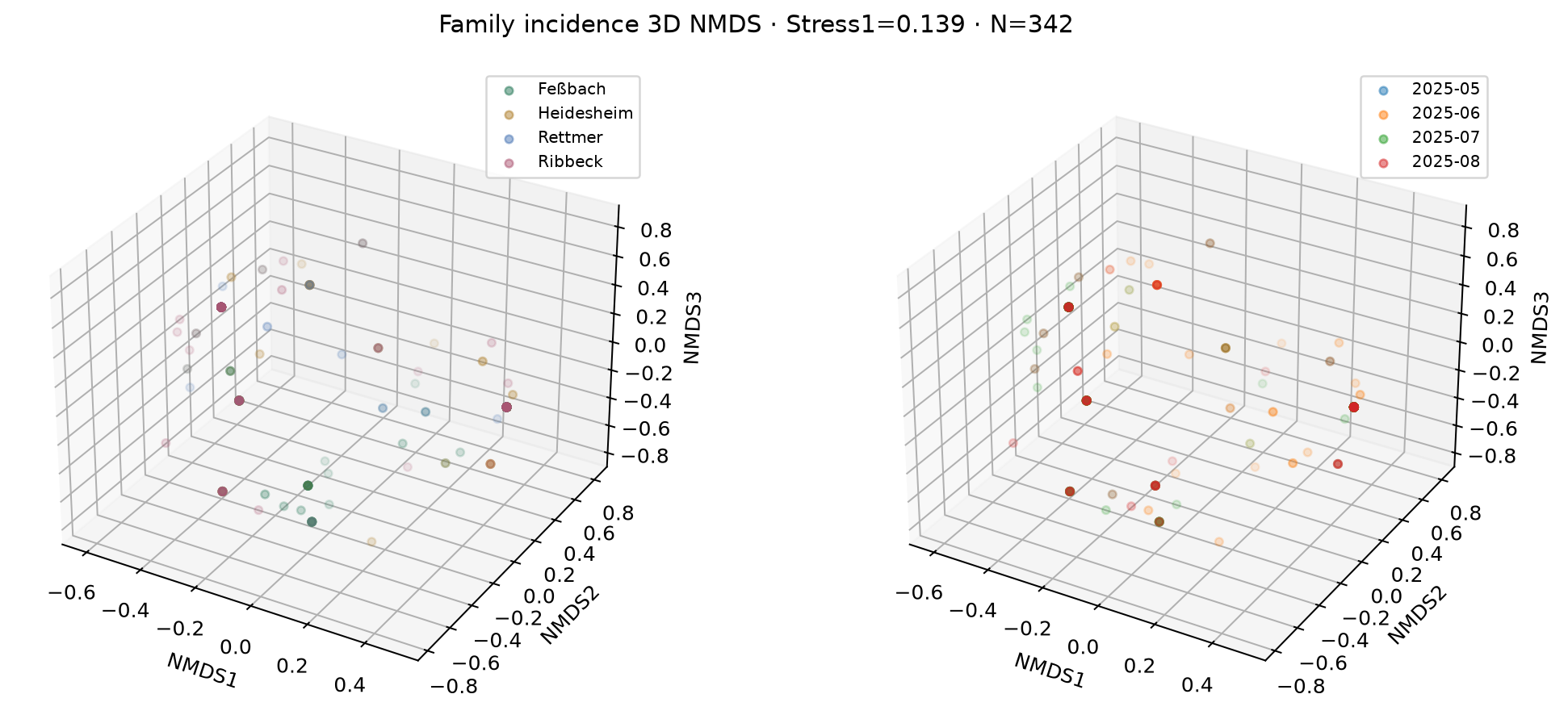
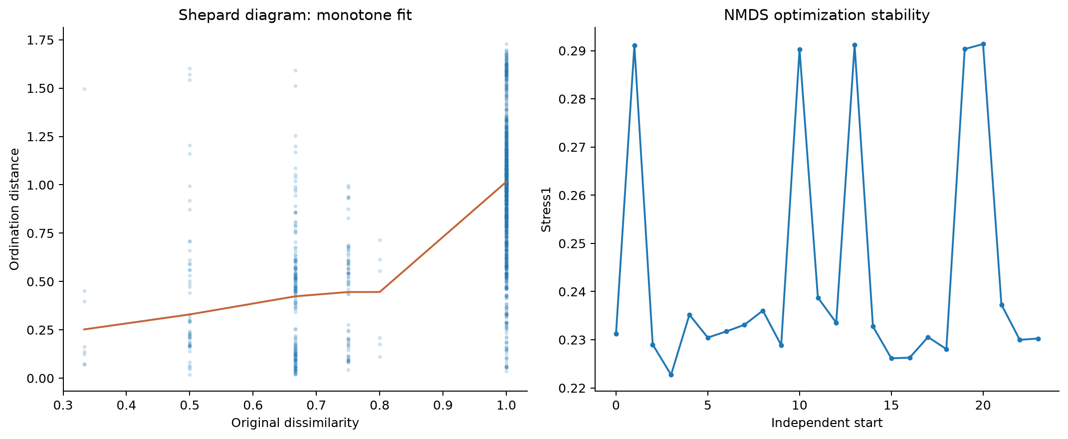
2D Stress1 is 0.223 (incidence) and 0.218 (area), limiting detailed geometric interpretation. The 3D fits improve to 0.139 and 0.135. Site and campaign colors overlap substantially. Use family frequencies and pairwise dissimilarities alongside the plots; NMDS axes have no biological units.
Click a point to inspect every coincident photo. The 3D view is an orthographic projection of the 3D fit; rotation changes the view, not the embedding.
Static NMDS figures and optimization diagnostics2D family incidence NMDS; coincident points represent identical observed family sets. Download SVG2D conditional family-area NMDS; no-family photos are excluded. Download SVG3D incidence NMDS, showing the same fit colored by site and month. Download SVGShepard diagram and start-wise Stress1 for the 2D incidence NMDS. The line is the monotone fitted disparity. Download SVG
The implementation uses weighted strong-tie nonmetric SMACOF: equal dissimilarities receive equal fitted disparities. Exact duplicate profiles are collapsed and weighted by photo multiplicities. Twenty-four starts are used in 2D and twelve in 3D; Stress1 is normalized residual distance error. This custom implementation is not a claim that vegan was executed. Strong-tie handling and the absence of step-across differ from some ecological defaults; see vegan’s NMDS guidance for the implications of high dissimilarities and tied distances. Start-wise diagnostics and coordinates are exported.
5. Shared DINO PCA and structural α, β, γ
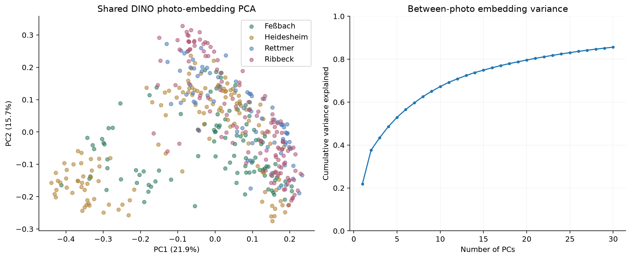
One PCA is fitted to all 439 photo means in the same 768-dimensional DINOv3 coordinate system. Every eligible full-frame patch is unit-normalized before averaging; the resulting photo means retain their lengths. PCA is centered, without whitening. This is a between-photo PCA; within-photo variation is retained separately in Rao Q.
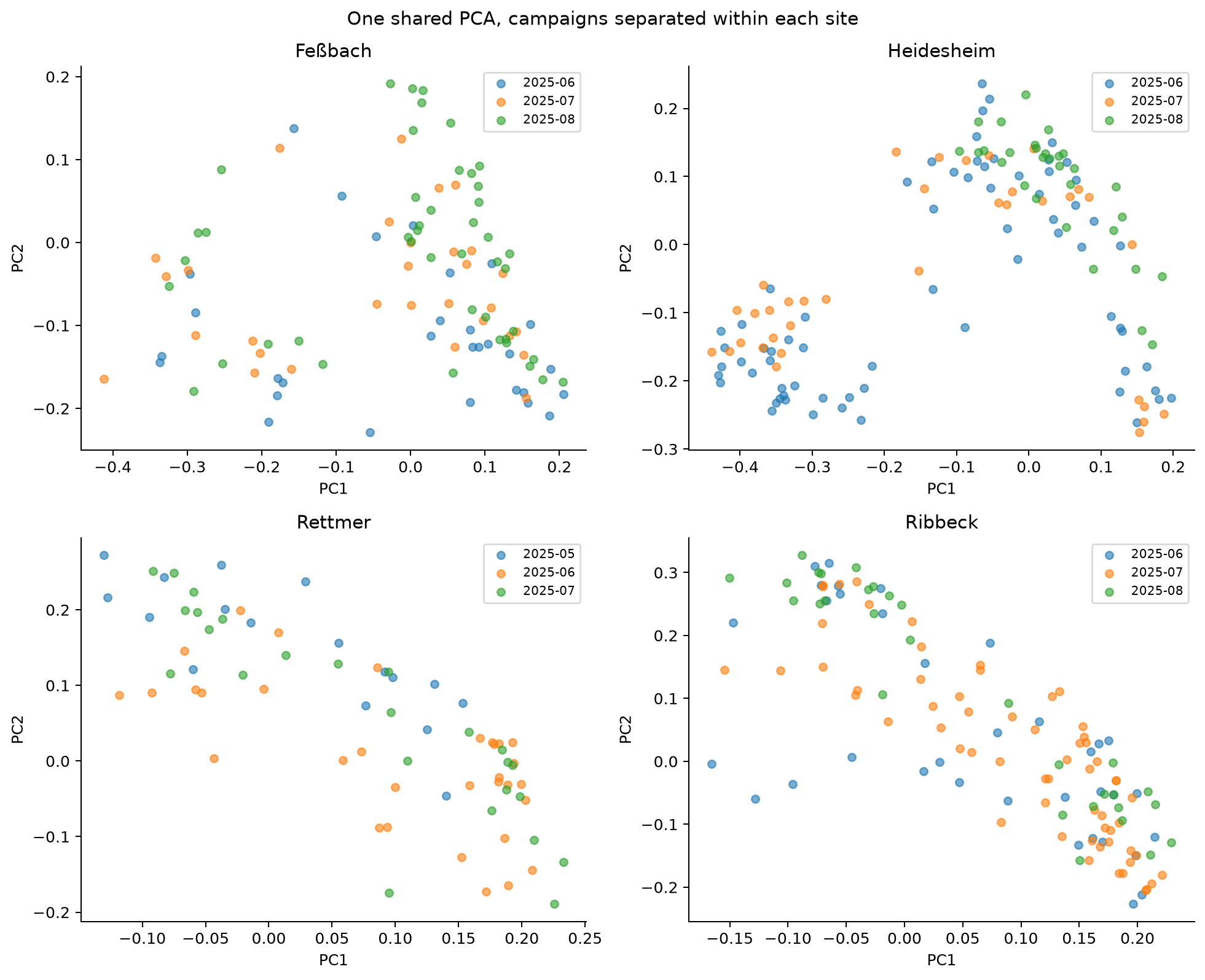
Shared 439-photo DINO PCA and cumulative explained variance; photo means are not renormalized. Download SVGSame shared PCA coordinates within each site, colored by month. Download SVG
PC1 explains 21.9% and PC2 15.7% of between-photo variance (37.6% together). Inspection of representative photos suggests PC1 runs from dry vegetation or exposed ground toward green canopies. PC2 also reflects apparent canopy density, ground visibility and camera framing. These are visual interpretations of examples, not independently validated structural traits. Viewpoint, illumination, plant condition and taxonomic composition can all contribute.
Photographs at seven quantiles of shared PC1. Low to high follows the fitted axis, not a botanical scoring rubric. Download SVGPhotographs at seven quantiles of shared PC2. Framing and apparent ground or canopy visibility contribute. Download SVG
An exact continuous-feature diversity partition
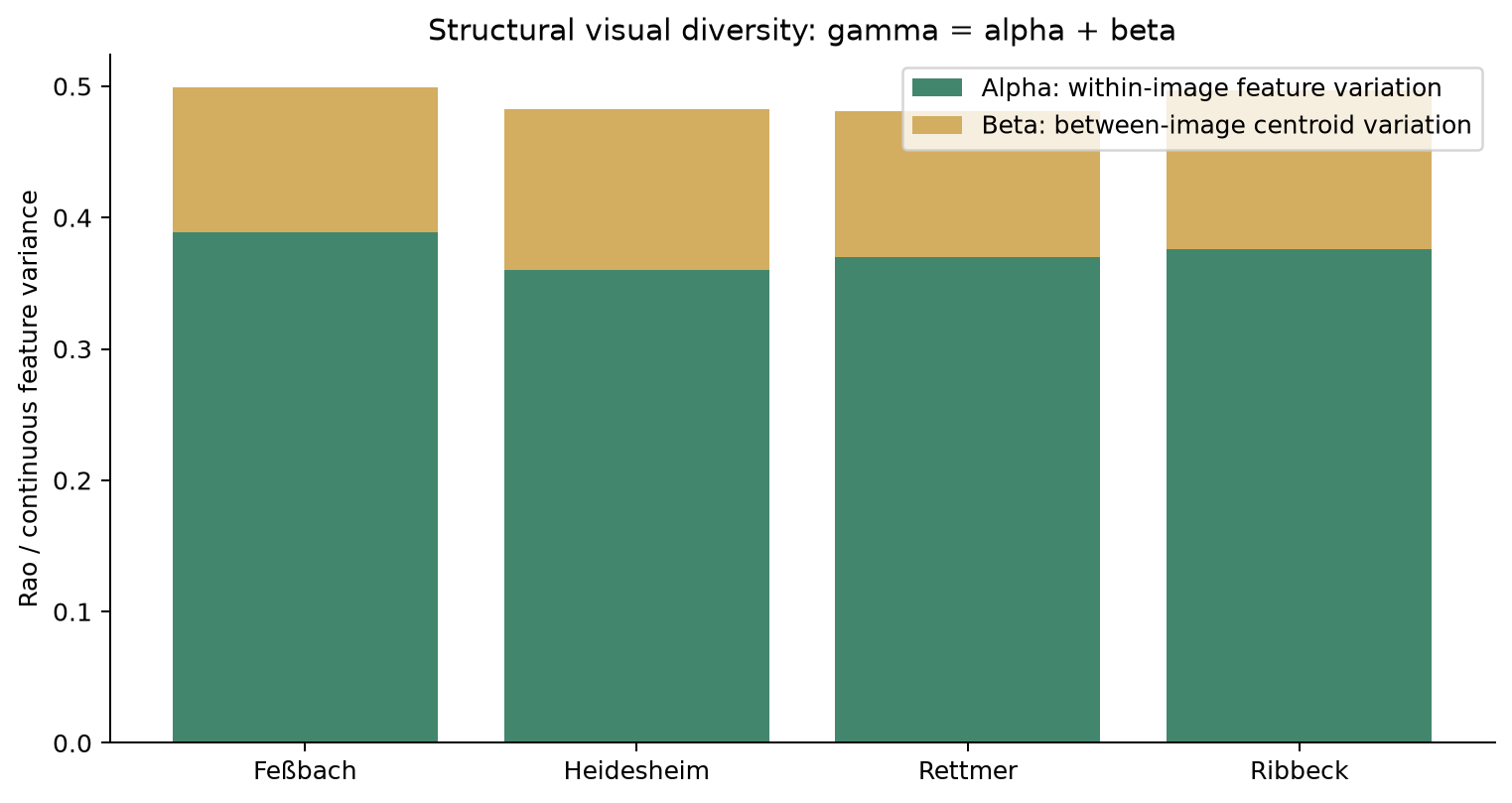
For unit patch features z: αᵢ = Qᵢ = 1 − ‖μᵢ‖² Group α = mean(Qᵢ) · β = mean(‖μᵢ − μ̄‖²) · γ = 1 − ‖μ̄‖² γ = α + β
Here μᵢ is a photo’s mean patch feature and μ̄ the equal-photo group mean. Q equals the expected cosine dissimilarity of two independently sampled eligible patches, including self-pairs. It is the quadratic diversity of these visual features; its exact variance identity avoids choosing cluster counts. The calculation uses all 768 dimensions, rather than the first two plotted PCs. The general dissimilarity-based framework is described by Rao (1982).
Site
α: within images
β: between images
γ = α + β
β / γ
Feßbach
0.389
0.110
0.499
22.1%
Heidesheim
0.360
0.122
0.482
25.4%
Rettmer
0.370
0.112
0.481
23.2%
Ribbeck
0.376
0.121
0.497
24.4%
Exact continuous visual diversity: mean within-photo α plus between-photo β equals pooled γ. Download SVG
Across all sites, α = 0.3730, β = 0.1306 and γ = 0.5035. The hierarchical partition assigns 74.1% of total feature diversity to variation within photos, 23.3% to variation between photos within sites, and 2.6% to differences between site centroids. Among between-photo variation alone, site centroids account for 10.2%. Most visual diversity therefore occurs within sites and photographs. This descriptive partition is not a significance test or an effect of management.
Earlier structural ranking and finalized local clustering decisions
The earlier composite averages cohort percentile ranks of Rao Q, nearest-neighbor intrinsic dimensionality (L2N2), and persistent Leiden cluster count. It used ten deterministic 250-patch resamples per image (five graph evaluations), with 1,000 rank bootstraps and alternative component weights. The report exposes that ranking and its stored rank interval as a sensitivity view. The primary new Q score uses every eligible patch and can order images differently.
The previous chat, Image analysis experiment with DINO x AnyUp, finalized local crop fractions of 5% and 10%, 75% overlap, four inverse-aligned flips, bilinear interpolation and Hann blending, with no AnyUp. Both automatic K-means and full-covariance GMM were retained. GMM selects K from 1–12 by −2 log L + 4 pK log n; K-means uses spatial held-out silhouettes and a one-standard-error choice near K = 5. PCA and orthogonal PCA-varimax were retained for visualization; 3 and 16 PCs were tested. No additional unit normalization, whitening or XY clustering features were adopted in that local workflow.
Those local-clustering choices are preserved in the recovered protocol. The present common-coordinate, whole-frame Q/PCA analysis is a separate cached-feature calculation. The photo browser now adds the agreed 5% local-crop, K-means and λ=4 GMM comparison as a separate full-cohort batch, with completion status shown explicitly.
Evidence, limitations and reproducibility
Source identity is SHA-256 of original photo bytes. The five duplicated archive entries occur at Rettmer and are counted once; their aliases are retained. The source archive prefix is 2025/Annotation Indicator/Plot view/all_farms_plot/. All input IDs, 439 hashes, campaigns and metadata matches are in the dataset inventory. The source results and selection exports match the audited server versions.
Taxonomic support 0.7 combines the existing crop-quality/context support and the stored classifier adoption rules; it is not a calibrated 70% probability of correctness. Family, genus and species hypotheses are collapsed to the classifier’s recorded family lineage. Across the cohort this includes 263 direct family hypotheses, 155 genus hypotheses and 84 species hypotheses. For example, Rumex contributes to Polygonaceae and Malva moschata to Malvaceae. Promoted genus/species hypotheses account for 39.1% of the aggregated family-assigned pixel area. The aggregation was independently verified in all 439 photos. Order/class-only identifications cannot establish a family. Accepted mixed hypotheses share their source region area according to the earlier export. Relative area is an image-region proxy, not specimen abundance. The catalogue is preserved without a new botanical harmonization; labels such as Hydrophyllaceae and Boraginaceae remain distinct.
Raw DINOv3 ViT-B/16 patch features use facebook/dinov3-vitb16-pretrain-lvd1689m, pinned revision 5931719e67bbdb9737e363e781fb0c67687896bc. The working full frames were limited to 1,280 pixels on their longest side. Artifact-excluded and padded patches are omitted; there is no vegetation-only foreground mask. Some background therefore legitimately contributes to the reported visual diversity. Original thumbnails shown here still display annotation boards or plot frames that may be excluded from feature calculations.
Rare-family evidence to review before ecological interpretation
Family catalogue label
Photos
Inspect evidence
Hydrophyllaceae
1
Hypericaceae
1
Lamiaceae
1
Malvaceae
2
Plantaginaceae
2
Restionaceae
1
Scrophulariaceae
1
Thesiaceae
1
Urticaceae
2
These catalogue labels occur in at most two photos across all sites. Review their accepted regions against original photos and harmonize taxonomy before treating them as verified records. A large accumulation plateau can reflect limits of identification as well as limits of observed diversity.
The reproduction script reads the pinned cached run and metadata_join.json on the existing Linux analysis server and writes a separate report directory. It needs NumPy, SciPy, scikit-learn, Matplotlib and Pillow. Current full-cohort outputs do not train classifiers or regenerate taxonomic evidence. No ecological p-values are claimed because site, campaign, repeated plots, viewpoints and model-detection uncertainty are not independent controlled replicates.