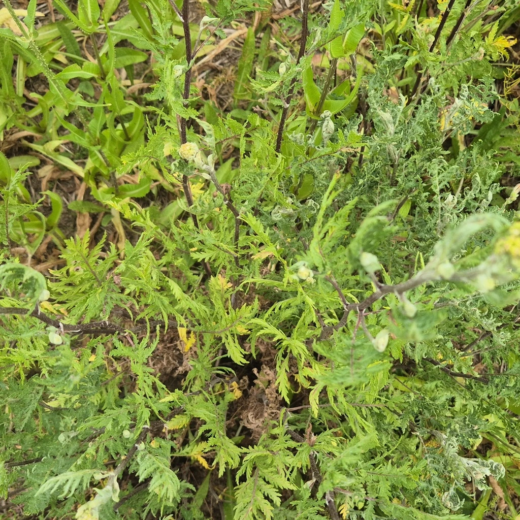
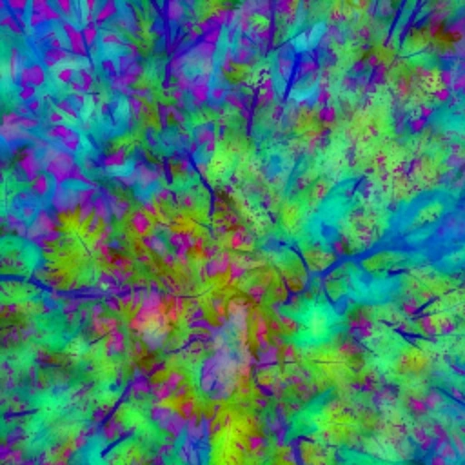
A leaf can occupy only a few model patches in a complex meadow. Local clipping enlarges that structure in the model’s field of view, then brings overlapping observations back into one continuous feature map.
The DINOv3 encoder stays fixed. Our workflow changes the scale and surrounding context supplied to it; it does not alter the transformer’s learned attention weights.
Overlapping local windows 5% or 10% of the working image’s short side→
→A continuous feature field Four flips · 75% overlap · weighted blending
Crop boxes illustrate the process, rather than an annotation or a selected organism. The final false-color map is an actual completed analysis.
01
Clip locally
Set the square crop side to 5% or 10% of the working short side. Move it at about one quarter of its width: neighboring windows overlap by about 75%. Include edge windows so the image is covered.
Local focus reduces the scene surrounding a feature. It gives fine structures more model patches while preserving their immediate neighborhood.
02
Enlarge and encode
Resize each crop to 384 × 384 with bicubic interpolation. A 16 × 16 model patch then spans a smaller area of the original photograph; the crop produces a 24 × 24 token grid.
Convert RGB values to 0–1 and apply the checkpoint’s mean/std normalization. Enlargement reallocates model resolution; it does not create new optical detail.
03
Align four views
Encode the original, horizontal flip, vertical flip, and both flips. Undo each flip on the spatial token map and average corresponding feature vectors before projecting them.
Alignment ensures the same image locations are combined. Averaging reduces dependence on orientation and the crop’s position relative to the model grid.
04
Blend the overlaps
Interpolate each projected token map onto its crop window. Weight it with a separable Hann window, floored at 0.05, and sum contributions at their original coordinates.
Divide by the accumulated weights at every location. Crop centers contribute more than crop borders, softening lattice-like seams. AnyUp is not part of this workflow.
02 / MAKE THE FEATURES VISIBLE
Color is a view into feature space.
The map is a visualization of learned features. Its colors are not taxonomic identities, and a color boundary is not automatically a biological object boundary.
PCA
Reduce the 768-dimensional features to 16 retained axes. PCA scores retain their scale: this experiment uses no whitening or additional explicit unit-vector normalization. Display three axes as red, green, and blue.
PCA–varimax
Rotate the retained basis orthogonally: Brot = BR and Xrot = XR, with RᵀR = I. Varimax encourages simpler loadings. Three rotated axes form the displayed colors.
The 16-dimensional subspace and Euclidean distances remain unchanged. This rotation changes interpretability and color appearance, rather than adding information.
A common clustering space
Both clustering methods use all 16 scores, rather than the rendered RGB colors. There are no XY coordinate features or vegetation scoring masks. Independent color stretches and rotations mean hues need not match across methods.
03 / REGULATE THE NUMBER OF GROUPS
Enough complexity. A cost for excess.
We retain automatic K-means and full-covariance Gaussian mixtures. The selected number depends on the image’s feature distribution and the method’s preference for simplicity.
Automatic K-means
Test K = 3…12 using spatial-fold silhouette scores. Among candidates within one standard error of the best score, choose the count closest to five. The final fit uses up to 8,192 sampled locations, ten initializations, and seed 42.
K-means minimizes within-group squared distances. It does not impose equal group areas. The preference toward five is explicit; it is not entirely preference-free selection.
GMM · strengthened BIC · λ=4
Fit full-covariance mixtures for K = 1…12 on the same sample. Select the converged model with the lowest penalized score, breaking an exact tie toward smaller K.
Sλ(K) = −2 log LK + λ pK log n
For d dimensions, pK = K[d + d(d+1)/2] + K − 1. At d=16 this is 153K − 1 parameters. λ=1 is ordinary BIC; our choice λ=4 charges four times the usual complexity penalty.
Full covariance allows correlated, elongated groups. The fits use covariance regularization 10−5, three initializations, seed 42, and tolerance 0.001. λ is a model-selection penalty, distinct from a Bayesian concentration prior.
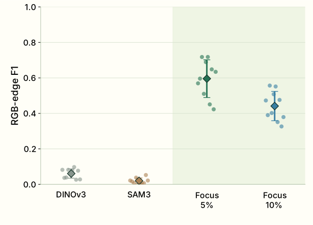
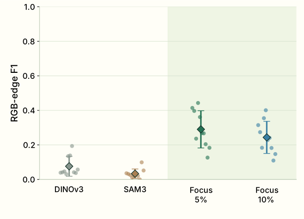
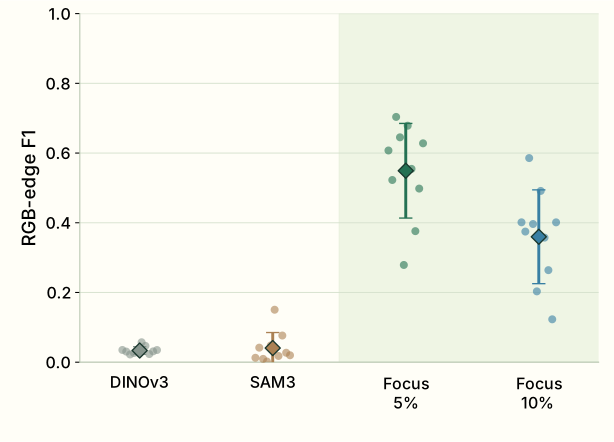
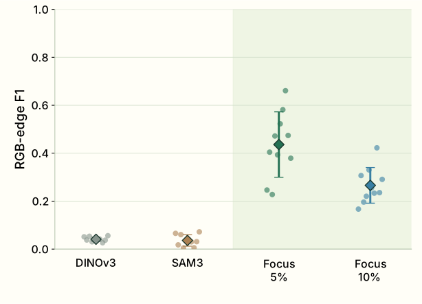
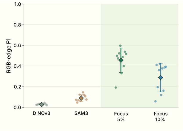
RGB-edge F1 · mean ± sample SD · ten photographs per dataset
Dataset
DINOv3
SAM3
Our focus 5%
Our focus 10%
Vegetation
0.061 ± 0.026
0.020 ± 0.016
0.596 ± 0.106
0.441 ± 0.083
Fungal networks
0.076 ± 0.057
0.034 ± 0.027
0.290 ± 0.108
0.244 ± 0.093
Aerial ecosystems
0.034 ± 0.011
0.041 ± 0.044
0.549 ± 0.136
0.360 ± 0.135
Coralscapes
0.041 ± 0.010
0.036 ± 0.024
0.436 ± 0.136
0.266 ± 0.074
Aquatic microscopy
0.028 ± 0.007
0.090 ± 0.032
0.456 ± 0.118
0.288 ± 0.138
What is this F1 score measuring?
Edges in the photograph
Convert RGB to luminance, apply Gaussian smoothing (σ=1), and calculate Sobel gradient magnitude. The strongest 15% of eligible gradients form the fixed appearance reference. Exclude a two-pixel image margin.
Extract predicted boundaries where neighboring partition labels differ. Precision is the fraction of predicted boundary pixels near reference edges; recall is the fraction of reference edge pixels near a prediction. Matching uses a Manhattan distance of two working-image pixels.
Every photograph receives one score. Summaries give every photograph equal weight; dots are individual scores and whiskers are sample SD, rather than confidence intervals.
A controlled focus comparison
The DINOv3 and local-focus partitions use the same fixed K-means count of six, sixteen PCA axes, matched fitting locations, and independent cluster centers. This holds the clustering count constant while comparing feature extraction.
Local 5% and 10% use enlarged crops, four-flip averaging, approximately 75% overlap, and Hann blending. SAM3 uses automatic mask generation with no user-supplied text, points, boxes, or object requests.
These frozen benchmark scores precede the automatic K selection described above. They do not evaluate the later GMM λ=4 or automatic K-means partitions. The sampled collection is illustrative, and the five-domain result is specific to this appearance metric.
Annotated class boundaries: SAM3 leads on Coralscapes
Among these five datasets, only Coralscapes has eligible pixel-level class boundaries for this comparison. Its mean annotated-boundary F1 is SAM3: 0.113; DINOv3: 0.022; focus 5%: 0.038; focus 10%: 0.047. SAM3 leads that class-boundary measure.
RGB texture edges also include internal organism detail, shadows, and substrate texture. Consequently, the strong fine-detail advantage shown above does not establish superior biological segmentation. Missing references for the other four domains are unavailable values, not zero scores.
5% is the finer, more expensive view; 10% retains a broader neighborhood with fewer crops. The model supplies features, while the biological question determines which structures and groupings are useful.